An Interactive Introduction to Multi-Task Learning

Introduction

Figure 1: Multitasking may be difficult for us, but it can make machine learning models smarter. Image courtesy of decisions

A couple of years ago, I was working on a music recommendation system for a small contract. The system weighed if somebody would click on a song and if they would actually finish listening to it. To integrate Machine Learning (ML) into such a system, the seemingly obvious answer would be to train two separate models to handle each of these tasks. But when you’re working with a small set of data–especially on a more niche task like this–it can simply be impossible to train two models from the ground up that are actually accurate. That’s when I learned about Multi-Task Learning (MTL).

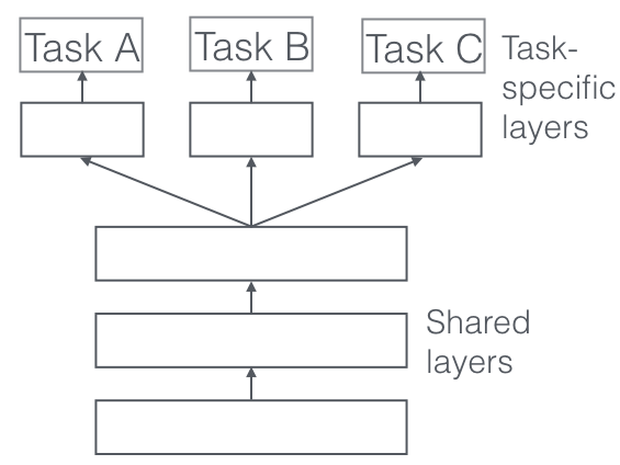
MTL has become one of the most interesting subfields of ML for me. Instead of training separate models for separate tasks, you train one model that learns to do multiple related things simultaneously. The model shares most of its parameters across tasks, only splitting apart near the end to make predictions on a task-by-task basis (see the visualization below).

Figure 2: Hard Parameter Sharing: The model learns a shared representation before branching out for specific tasks. Image courtesy of ruder.io

It sounds a little weird. Wouldn’t models perform better if you trained them with a focus on a particular task? Doesn’t training on multiple tasks just confuse a model?

It turns out that, when you are working on solving tasks that are closely related, using MTL can greatly improve performance on both (or all 10) tasks! This is because similar tasks often depend on the same underlying patterns. A model that has been forced to solve both tasks has to learn these shared patterns. MTL can essentially act as a form of regularization¹. It can’t “cheat” (or overfit) by memorizing features, and it is encouraged to learn the deeper meaning behind given inputs.

Figure 3: It can help to think of ML models like dogs when understanding Multi-Task Learning (MTL). Image courtesy of ChatGPT

Think about it like teaching a dog a bunch of tricks at the same time. Naturally, it is a lot easier to teach a dog their fourth or fifth trick than to teach their first or second trick. This is because the dog has learned the basic underlying patterns or skills that can be transferred across all tricks. Particularly, the ability to pay attention and control their impulses.

If a dog were able to practice multiple commands together, the dog gets better at that underlying skill of focus and self-control.

Figure 4: Tasks can conflict, causing them to “fight” for better performance!

But, like all things in ML, multi-task learning is a lot harder than it looks.

The biggest problem in this field is when tasks fight each other. The model gets worse at both compared to training them separately. Sometimes one task dominates the training and the other barely learns anything. Sometimes everything works fine for 50 epochs and then suddenly collapses. This concept is known as negative transfer.

This was frustrating for me because, once you understand it, the core idea feels so intuitive. Of course related tasks should help each other. Of course sharing knowledge would make the learning more efficient. But making it work in practice requires understanding what’s happening internally in these models.

In this article, we’ll look at when multi-task learning helps, when it fails, and what you can do to make it work. It does have its struggles, but it remains one of the most elegant ideas in machine learning.

Defining Multi-Task Learning

Let’s start with the simplest possible definition.

Multi-task learning is when you train a single model to solve multiple related problems at the same time using shared internal representations.

That’s it. But we should try and understand what that really means 😊

Basic Setup

Say you have three tasks: Task A, Task B, and Task C. In traditional machine learning, you’d train three separate models.

• Model A would learn from data labeled for Task A
• Model B would learn from data labeled for Task B
• Model C would learn from data labeled for Task C

flowchart LR
  I[(Input x)]

  subgraph A["Model A (θ_A)"]
    A1[Encoder / Layers] --> A2[Head A] --> OA[(ŷ_A)]
  end
  subgraph B["Model B (θ_B)"]
    B1[Encoder / Layers] --> B2[Head B] --> OB[(ŷ_B)]
  end
  subgraph C["Model C (θ_C)"]
    C1[Encoder / Layers] --> C2[Head C] --> OC[(ŷ_C)]
  end

  I --> A1
  I --> B1
  I --> C1

  style A fill:#f2f2f2,stroke:#c9c9c9,color:#222
  style B fill:#f2f2f2,stroke:#c9c9c9,color:#222
  style C fill:#f2f2f2,stroke:#c9c9c9,color:#222

Figure 5: The traditional approach is to use single task learning. Three separate models are trained independently for Tasks A, B, and C. Diagram courtesy of me.

Each model has its own parameters (the weights and connections inside the neural network). They don’t talk to each other. They don’t share anything.

In Multi-task learning, you train one model that has two kinds of parameters. The first kind is Shared Parameters, written as {\theta}_shared. These are parameters used by all tasks. They serve as the common foundation for the whole model.

The second kind of parameter is task-specific parameters, written as ({\theta}_A, {\theta}_B, {\theta}_C). These are unique to each task

flowchart LR
  I[(Input x)]

  subgraph S["Shared Trunk (θ_shared)"]
    S1[Shared Encoder / Layers] --> S2[Shared Representation h]
  end

  subgraph TA["Task A Head (θ_A)"]
    A1[Head A] --> OA[(ŷ_A)]
  end
  subgraph TB["Task B Head (θ_B)"]
    B1[Head B] --> OB[(ŷ_B)]
  end
  subgraph TC["Task C Head (θ_C)"]
    C1[Head C] --> OC[(ŷ_C)]
  end

  I --> S1
  S2 --> A1
  S2 --> B1
  S2 --> C1

  style S fill:#eef6ff,stroke:#8fb7e8,color:#1f3a5f
  style TA fill:#f2f2f2,stroke:#c9c9c9,color:#222
  style TB fill:#f2f2f2,stroke:#c9c9c9,color:#222
  style TC fill:#f2f2f2,stroke:#c9c9c9,color:#222

Figure 6: Multi-task learning with shared parameters and task-specific heads. Diagram courtesy of me.

The model processes input through the shared layers first. These layers learn features that help with all the tasks. Then the network splits, and each task gets its own set of final layers to make its specific prediction.

Optimization

We’re going to get slightly more formal here (but trust me when I say it’s simpler than it looks).

When you train a model for a single task, you’re minimizing one loss function. The loss measures how wrong your predictions are. Lower loss essentially means better predictions.

When you train a multi-task model, you’re minimizing a combined loss that includes all your tasks.

\min_{\theta_{\text{shared}}, \theta_A, \theta_B, \theta_C} \left[ w_A \cdot \mathcal{L}_A + w_B \cdot \mathcal{L}_B + w_C \cdot \mathcal{L}_C \right]

Here, \mathcal{L}_A, \mathcal{L}_B, \mathcal{L}_C are the individual loss functions for each task. w_A, w_B, w_C are weights that control how much each task matters (we’ll come back to why these are important later).

You’re trying to find one set of shared parameters that works well for all three tasks simultaneously

Another Way of Thinking About It

In case that was confusing, there’s another way we can think about this process that might be more intuitive for you.

Every machine learning model makes assumptions. It has to. There are infinite possible patterns in data, and the model needs some way to decide which patterns to pay attention to.

These assumptions are called inductive biases². They guide the model toward certain kinds of solutions.

When learning with a single task, the main inductive bias comes from your model architecture and regularization techniques. The model assumes that simpler explanations are better, that certain structures matter, etc.

In multi-task learning, you add another inductive bias. That is, the assumption that your tasks share common structure. The model is told that whatever it learns has to be useful for Task A AND Task B AND Task c.

This is a really helpful constraint. It forces the model to pick up on features that generalize well. If a pattern only helps with Task A but hurts Task B, then the model can’t rely on it in the shared layers. That’s because, if it does, then the loss goes up, and the model is focused on minimizing that loss.

flowchart LR
  H[All possible models / hypotheses]

  subgraph ST["Single-task (Task A only)"]
    SA[Many models can fit Task A]
    SQ["Includes real patterns and quirks of dataset (overfitting)"]
  end

  subgraph MT["Multi-task (Task A and Task B)"]
    MA[Models that fit Task A]
    MB[Models that fit Task B]
    INT[Overlap: models that fit both tasks]
    GEN[Higher chance of learning shared structure]
  end

  H --> SA
  SA --> SQ

  H --> MA
  H --> MB
  MA --> INT
  MB --> INT
  INT --> GEN

  style ST fill:#fff5e8,stroke:#e4b46a,color:#3f2b0c
  style MT fill:#eef6ff,stroke:#8fb7e8,color:#1f3a5f
  style INT fill:#d7ecff,stroke:#4f88c6,color:#123a63

Figure 7: A model of multi-task learning based on inductive bias. Requiring one model to satisfy multiple tasks forces it to select features that fit both tasks’ criteria. This causes it to learn more robust and important features. Diagram courtesy of me.

Think of it this way. When you train on Task A alone, there are many possible models that could achieve good performance (i.e., low loss). Some of these possible models learn actual patterns. Some of them just memorize things unique to your training data. Of course, the former is much better. The latter will often lead to overfitting³.

When you train on Task A and Task B together, far fewer models will work well for both. The methods that survive both are the ones that learned real underlying patterns. That is, something fundamental enough that can transfer across both tasks. It is a lot harder to overfit to the training data (i.e., memorize quirks that are specific to the training set) when you’re focusing on separate tasks.

Hopefully this second perspective is a lot more intuitive and easier to understand. This is how I first grasped MTL and the beauty behind it. I call this the “Inductive Bias Perspective”

Examples of Where it Helps

I’m going to show you a simple example where MTL clearly outperforms single task learning. We’ll use a simple problem where we control how related the tasks are. This lets us see the effect without all the noise of a real-world dataset. Since the point of this blog post is to learn, this should be enough for our purposes.

Setting Up Two Related Tasks

You have data where each input has some hidden structure. Two tasks both depend on parts of that hidden structure in slightly different ways.

Our scenario is as follows: - Input: Some features x - Hidden truth: There’s a shared underlying factor z_shared and two private factors z_A and z_B. - Task A: Predict y_A = z_{\text{shared}} + z_A + \text{noise} - Task B: Predict y_B = z_{\text{shared}} + z_B + \text{noise}

Both tasks depend on the same shared factor. If a model can learn to extract z_{\text{shared}}, it helps with both tasks. We can generate the data and see what happens using Python and PyTorch.

import numpy as np
import torch
import torch.nn as nn
import torch.optim as optim
import plotly.graph_objects as go
from plotly.subplots import make_subplots

# Set random seeds for reproducibility
np.random.seed(100)
torch.manual_seed(100)

# Generate synthetic data
n_samples = 1000
n_features = 20

# Create input features
X = np.random.randn(n_samples, n_features)

# Create hidden shared and private factors
z_shared = X[:, 0] + 0.5 * X[:, 1]  # Shared underlying pattern
z_private_A = X[:, 2] + 0.3 * X[:, 3]  # Task A's private pattern
z_private_B = X[:, 4] + 0.3 * X[:, 5]  # Task B's private pattern

# Create targets for a strongly related-task setting:
# both tasks are mostly driven by the same shared factor.
y_A = z_shared + 0.1 * z_private_A + np.random.randn(n_samples) * 0.5
y_B = z_shared + 0.1 * z_private_B + np.random.randn(n_samples) * 0.5

# Split into train and test
split = 800
X_train, X_test = X[:split], X[split:]
y_A_train, y_A_test = y_A[:split], y_A[split:]
y_B_train, y_B_test = y_B[:split], y_B[split:]

# Convert to PyTorch tensors
X_train_t = torch.FloatTensor(X_train)
X_test_t = torch.FloatTensor(X_test)
y_A_train_t = torch.FloatTensor(y_A_train).reshape(-1, 1)
y_A_test_t = torch.FloatTensor(y_A_test).reshape(-1, 1)
y_B_train_t = torch.FloatTensor(y_B_train).reshape(-1, 1)
y_B_test_t = torch.FloatTensor(y_B_test).reshape(-1, 1)

print(f"Training samples: {len(X_train)}")
print(f"Test samples: {len(X_test)}")
print(f"Input features: {n_features}")

Training samples: 800
Test samples: 200
Input features: 20

Single Task Models

First let’s train two separate models. Each one only sees data for its own task.

class SingleTaskModel(nn.Module):
    def __init__(self, input_size, hidden_size=64):
        super().__init__()
        self.network = nn.Sequential(
            nn.Linear(input_size, hidden_size),
            nn.ReLU(),
            nn.Linear(hidden_size, hidden_size),
            nn.ReLU(),
            nn.Linear(hidden_size, 1)
        )
    
    def forward(self, x):
        return self.network(x)

def train_single_task(model, X_train, y_train, X_test, y_test, epochs=100):
    optimizer = optim.Adam(model.parameters(), lr=0.001)
    criterion = nn.MSELoss()
    
    train_losses = []
    test_losses = []
    
    for epoch in range(epochs):
        # Training
        model.train()
        optimizer.zero_grad()
        predictions = model(X_train)
        loss = criterion(predictions, y_train)
        loss.backward()
        optimizer.step()
        train_losses.append(loss.item())
        
        # Testing
        model.eval()
        with torch.no_grad():
            test_pred = model(X_test)
            test_loss = criterion(test_pred, y_test)
            test_losses.append(test_loss.item())
    
    return train_losses, test_losses

# Train separate models (fixed init seeds for fair comparison)
torch.manual_seed(1100)
model_A = SingleTaskModel(n_features)
torch.manual_seed(1200)
model_B = SingleTaskModel(n_features)

print("Training model for Task A")
train_A, test_A = train_single_task(model_A, X_train_t, y_A_train_t, X_test_t, y_A_test_t)

print("Training model for Task B")
train_B, test_B = train_single_task(model_B, X_train_t, y_B_train_t, X_test_t, y_B_test_t)

print(f"\nFinal test MSE on Task A (single): {test_A[-1]:.4f}")
print(f"Final test MSE on Task B (single): {test_B[-1]:.4f}")

Training model for Task A
Training model for Task B

Final test MSE on Task A (single): 0.2845
Final test MSE on Task B (single): 0.3471

Multi-Task Models

Now let’s build one model that learns both tasks together. It has shared layers that both tasks use. It then splits into heads for each task.

class MultiTaskModel(nn.Module):
    def __init__(self, input_size, hidden_size=64):
        super().__init__()
        # Shared layers
        self.shared = nn.Sequential(
            nn.Linear(input_size, hidden_size),
            nn.ReLU(),
            nn.Linear(hidden_size, hidden_size),
            nn.ReLU()
        )
        
        # Task heads
        self.head_A = nn.Linear(hidden_size, 1)
        self.head_B = nn.Linear(hidden_size, 1)
    
    def forward(self, x):
        # Everyone goes through shared layers first
        shared_features = self.shared(x)
        
        # We split to make predictions for each task
        out_A = self.head_A(shared_features)
        out_B = self.head_B(shared_features)
        return out_A, out_B

def train_multi_task(model, X_train, y_A_train, y_B_train, X_test, y_A_test, y_B_test, epochs=100):
    optimizer = optim.Adam(model.parameters(), lr=0.001)
    criterion = nn.MSELoss()
    
    train_losses_A = []
    train_losses_B = []
    test_losses_A = []
    test_losses_B = []
    
    for epoch in range(epochs):
        # Training
        model.train()
        optimizer.zero_grad()
        pred_A, pred_B = model(X_train)
        
        loss_A = criterion(pred_A, y_A_train)
        loss_B = criterion(pred_B, y_B_train)
        
        # Average keeps gradient scale comparable to single-task training
        total_loss = (loss_A + loss_B) / 2
        total_loss.backward()
        optimizer.step()
        
        train_losses_A.append(loss_A.item())
        train_losses_B.append(loss_B.item())
        
        # Testing
        model.eval()
        with torch.no_grad():
            test_pred_A, test_pred_B = model(X_test)
            test_loss_A = criterion(test_pred_A, y_A_test)
            test_loss_B = criterion(test_pred_B, y_B_test)
            test_losses_A.append(test_loss_A.item())
            test_losses_B.append(test_loss_B.item())
    
    return train_losses_A, train_losses_B, test_losses_A, test_losses_B

# Train MTL model (fixed init seed for fair comparison)
torch.manual_seed(1300)
model_mtl = MultiTaskModel(n_features)

print("Training multi-task model...")
train_mtl_A, train_mtl_B, test_mtl_A, test_mtl_B = train_multi_task(
    model_mtl, X_train_t, y_A_train_t, y_B_train_t, X_test_t, y_A_test_t, y_B_test_t
)

print(f"\nFinal test MSE on Task A (multi-task): {test_mtl_A[-1]:.4f}")
print(f"Final test MSE on Task B (multi-task): {test_mtl_B[-1]:.4f}")
print(f"\nImprovement on Task A: {((test_A[-1] - test_mtl_A[-1]) / test_A[-1] * 100):.1f}%")
print(f"Improvement on Task B: {((test_B[-1] - test_mtl_B[-1]) / test_B[-1] * 100):.1f}%")

Training multi-task model...

Final test MSE on Task A (multi-task): 0.2593
Final test MSE on Task B (multi-task): 0.3167

Improvement on Task A: 8.9%
Improvement on Task B: 8.8%

Results

# Create interactive comparison plot
fig = make_subplots(
    rows=1, cols=2,
    subplot_titles=('Task A Test Loss', 'Task B Test Loss')
)

# Task A comparison
fig.add_trace(
    go.Scatter(y=test_A, name='Single-Task A', 
               line=dict(color='#e74c3c', width=2)),
    row=1, col=1
)
fig.add_trace(
    go.Scatter(y=test_mtl_A, name='Multi-Task A', 
               line=dict(color='#3498db', width=2)),
    row=1, col=1
)

# Task B comparison
fig.add_trace(
    go.Scatter(y=test_B, name='Single-Task B', 
               line=dict(color='#e74c3c', width=2, dash='dash')),
    row=1, col=2
)
fig.add_trace(
    go.Scatter(y=test_mtl_B, name='Multi-Task B', 
               line=dict(color='#3498db', width=2, dash='dash')),
    row=1, col=2
)

fig.update_xaxes(title_text="Epoch", row=1, col=1)
fig.update_xaxes(title_text="Epoch", row=1, col=2)
fig.update_yaxes(title_text="Mean Squared Error", row=1, col=1)
fig.update_yaxes(title_text="Mean Squared Error", row=1, col=2)

fig.update_layout(
    height=400,
    showlegend=True,
    hovermode='x unified'
)

fig.show()

Figure 8: Comparing single-task and multi-task learning performance over training

Look at those curves! The multi-task model (blue) consistently achieves lower test error than the single-task models (red) for both tasks.

This is because the multi-task model is being forced to learn the shared structure. Remember, both y_A and y_B depend on z_{\text{shared}}. When the model trains on both tasks, it quickly figures out that there’s a common pattern worth extracting. The shared layers learn to capture z_{\text{shared}}, and the task heads learn to handle z_A and z_B.

The single-task models don’t have this advantage. Each one has to learn everything from scratch, including the shared structure. With only 800 training samples per task, they struggle to find the necessary patterns. This is because we added noise earlier!

Why It Works (Data Efficiency)

We can also look at this from the angle of data efficiency. The multi-task model effectively gets more data.

It doesn’t literally have more samples. But because both tasks provide information about z_{\text{shared}}, the model learns that shared structure more reliably. It’s almost like having 1,600 training examples for learning the shared pattern. Meanwhile the separated model only has 800.

This is especially useful when you have very limited data. If you only have 100 training samples per task, then models training for specific tasks might barely learn anything. But the multi-task model can combine information across tasks and still find the important patterns.

The Biggest Issue with Multi-Task Learning

In the last example, we specifically set up the dataset so that tasks are related. They both depended on z_{\text{shared}}. But what happens if your tasks don’t actually share structure? Foreshadowing!

When Tasks Conflict

I’ll modify our setup to create tasks that do not share structure.

# Generate data where tasks conflict
np.random.seed(123)
torch.manual_seed(123)

n_samples = 1000
n_features = 20
X_conflict = np.random.randn(n_samples, n_features)

# Task A wants one pattern
z_A = X_conflict[:, 0] + 0.5 * X_conflict[:, 1]
y_A_conflict = z_A + np.random.randn(n_samples) * 0.1

# Task B wants a different pattern
z_B = -X_conflict[:, 0] + 0.8 * X_conflict[:, 2]  # Notice the negative sign
y_B_conflict = z_B + np.random.randn(n_samples) * 0.1

# Split data
split = 800
X_train_c = torch.FloatTensor(X_conflict[:split])
X_test_c = torch.FloatTensor(X_conflict[split:])
y_A_train_c = torch.FloatTensor(y_A_conflict[:split]).reshape(-1, 1)
y_A_test_c = torch.FloatTensor(y_A_conflict[split:]).reshape(-1, 1)
y_B_train_c = torch.FloatTensor(y_B_conflict[:split]).reshape(-1, 1)
y_B_test_c = torch.FloatTensor(y_B_conflict[split:]).reshape(-1, 1)

Now let’s train the same single task and multi-task models on this conflicting data.

# Train single-task models on conflicting tasks
model_A_conflict = SingleTaskModel(n_features)
model_B_conflict = SingleTaskModel(n_features)

train_A_c, test_A_c = train_single_task(
    model_A_conflict, X_train_c, y_A_train_c, X_test_c, y_A_test_c
)
train_B_c, test_B_c = train_single_task(
    model_B_conflict, X_train_c, y_B_train_c, X_test_c, y_B_test_c
)

# Train multi-task model on conflicting tasks
model_mtl_conflict = MultiTaskModel(n_features)
train_mtl_A_c, train_mtl_B_c, test_mtl_A_c, test_mtl_B_c = train_multi_task(
    model_mtl_conflict, X_train_c, y_A_train_c, y_B_train_c, 
    X_test_c, y_A_test_c, y_B_test_c
)

print(f"Task A - Single-task final test MSE: {test_A_c[-1]:.4f}")
print(f"Task A - Multi-task final test MSE: {test_mtl_A_c[-1]:.4f}")
print(f"Difference: {((test_mtl_A_c[-1] - test_A_c[-1]) / test_A_c[-1] * 100):+.1f}%\n")

print(f"Task B - Single-task final test MSE: {test_B_c[-1]:.4f}")
print(f"Task B - Multi-task final test MSE: {test_mtl_B_c[-1]:.4f}")
print(f"Difference: {((test_mtl_B_c[-1] - test_B_c[-1]) / test_B_c[-1] * 100):+.1f}%")

Task A - Single-task final test MSE: 0.0390
Task A - Multi-task final test MSE: 0.0471
Difference: +20.7%

Task B - Single-task final test MSE: 0.0350
Task B - Multi-task final test MSE: 0.0559
Difference: +60.0%

fig_conflict = make_subplots(
    rows=1, cols=2,
    subplot_titles=('Task A Test Loss', 'Task B Test Loss')
)

fig_conflict.add_trace(
    go.Scatter(y=test_A_c, name='Single-Task A', 
               line=dict(color='#27ae60', width=2)),
    row=1, col=1
)
fig_conflict.add_trace(
    go.Scatter(y=test_mtl_A_c, name='Multi-Task A', 
               line=dict(color='#e74c3c', width=2)),
    row=1, col=1
)

fig_conflict.add_trace(
    go.Scatter(y=test_B_c, name='Single-Task B', 
               line=dict(color='#27ae60', width=2, dash='dash')),
    row=1, col=2
)
fig_conflict.add_trace(
    go.Scatter(y=test_mtl_B_c, name='Multi-Task B', 
               line=dict(color='#e74c3c', width=2, dash='dash')),
    row=1, col=2
)

fig_conflict.update_xaxes(title_text="Epoch", row=1, col=1)
fig_conflict.update_xaxes(title_text="Epoch", row=1, col=2)
fig_conflict.update_yaxes(title_text="Mean Squared Error", row=1, col=1)
fig_conflict.update_yaxes(title_text="Mean Squared Error", row=1, col=2)

fig_conflict.update_layout(height=400, showlegend=True, hovermode='x unified')
fig_conflict.show()

Figure 9: Multi-task learning fails when tasks conflict

The multi-task model (red) does worse than the single task models (green). This is known as negative transfer. Negative transfer is the phenomenon where learning multiple tasks together actually hurts performance compared to training them separately. This is an unfortunately common scenario we come across when using multi-task learning.

Gradient Conflict

To understand why this happens we have to look at how neural networks fundamentally learn.

During training, the model computes gradients. A gradient tells you which direction to adjust each parameter to reduce the loss. If Task A’s loss is high, then its gradient points in the direction that would make Task A better.

This is really simple in single task learning. You have just one gradient, so you follow it!

But in multi-task learning, you can have multiple gradients. That is, one for each task. The problem is that those gradients might point in opposite directions.

The standard approach is to add the gradients together and move in that combined direction. But when the gradients point in opposite directions, they partially cancel out. You end up taking a tiny step. Oftentimes, that tiny step makes both tasks worse.

Visualizing Gradient Conflict

To better understand gradient conflict, we can look inside the model during training and watch the gradients.

def compute_gradient_conflict(model, X, y_A, y_B):
    """
    Compute the angle between gradients for Task A and Task B.
    Returns cosine similarity (1 = same direction, -1 = opposite, 0 = perpendicular)
    """
    criterion = nn.MSELoss()
    
    # Get predictions
    pred_A, pred_B = model(X)
    
    # Compute losses
    loss_A = criterion(pred_A, y_A)
    loss_B = criterion(pred_B, y_B)
    
    # Compute gradients for Task A
    model.zero_grad()
    loss_A.backward(retain_graph=True)
    grad_A = []
    for param in model.shared.parameters():
        if param.grad is not None:
            grad_A.append(param.grad.flatten().clone())
    grad_A = torch.cat(grad_A)
    
    # Compute gradients for Task B
    model.zero_grad()
    loss_B.backward()
    grad_B = []
    for param in model.shared.parameters():
        if param.grad is not None:
            grad_B.append(param.grad.flatten().clone())
    grad_B = torch.cat(grad_B)
    
    # Compute cosine similarity
    cos_sim = torch.dot(grad_A, grad_B) / (torch.norm(grad_A) * torch.norm(grad_B))
    
    return cos_sim.item()

# Track gradient conflict during training
def train_and_track_gradients(model, X_train, y_A_train, y_B_train, epochs=100):
    optimizer = optim.Adam(model.parameters(), lr=0.001)
    criterion = nn.MSELoss()
    
    gradient_similarities = []
    
    for epoch in range(epochs):
        # Compute gradient conflict before update
        if epoch % 5 == 0:  # Sample every 5 epochs
            cos_sim = compute_gradient_conflict(model, X_train, y_A_train, y_B_train)
            gradient_similarities.append(cos_sim)
        
        # Regular training step
        model.train()
        optimizer.zero_grad()
        pred_A, pred_B = model(X_train)
        
        loss_A = criterion(pred_A, y_A_train)
        loss_B = criterion(pred_B, y_B_train)
        total_loss = loss_A + loss_B
        
        total_loss.backward()
        optimizer.step()
    
    return gradient_similarities

# Compare gradient conflict
model_coop = MultiTaskModel(n_features)
model_conf = MultiTaskModel(n_features)

print("Training on cooperative tasks")
grad_sim_coop = train_and_track_gradients(model_coop, X_train_t, y_A_train_t, y_B_train_t)

print("Training on conflicting tasks...")
grad_sim_conf = train_and_track_gradients(model_conf, X_train_c, y_A_train_c, y_B_train_c)

Training on cooperative tasks
Training on conflicting tasks...

epochs_sampled = list(range(0, 100, 5))

fig_grad = go.Figure()

fig_grad.add_trace(go.Scatter(
    x=epochs_sampled,
    y=grad_sim_coop,
    name='Cooperative Tasks',
    line=dict(color='#3498db', width=3),
    mode='lines+markers'
))

fig_grad.add_trace(go.Scatter(
    x=epochs_sampled,
    y=grad_sim_conf,
    name='Conflicting Tasks',
    line=dict(color='#e74c3c', width=3),
    mode='lines+markers'
))

# Add reference lines
fig_grad.add_hline(y=0, line_dash="dash", line_color="gray", 
                   annotation_text="Perpendicular gradients")
fig_grad.add_hrect(y0=-1, y1=0, fillcolor="red", opacity=0.1, 
                   annotation_text="Conflict zone", annotation_position="top left")

fig_grad.update_layout(
    title="Cosine Similarity Between Task Gradients",
    xaxis_title="Epoch",
    yaxis_title="Gradient Cosine Similarity",
    yaxis_range=[-1.1, 1.1],
    height=450,
    hovermode='x unified'
)

fig_grad.show()

Figure 10: Gradient alignment during training: cooperative vs conflicting tasks

When tasks are well aligned with each other (blue line), their gradients mostly point in the same direction. Their cosine similarity stays positive, so the tasks are pulling the shared parameters in compatible directions. When tasks are conflicting (red line), the gradients usually point in opposite directions. The cosine similarity goes below zero.

This shows why multi-task learning does not perform well with conflicting tasks. The model is trying to satisfy both tasks at the same time. But since both tasks want different things, it ends up satisfying neither of them.

Better Understanding Task Similarity

I’ve created an interactive chart that shows how performance changes as task relatedness varies. Hover over the points to compare the models and gradient similarity at each relatedness value.

import plotly.graph_objects as go
from plotly.subplots import make_subplots

def generate_tasks_with_relatedness(relatedness, n_samples=1000, n_features=20, seed=100):
    np.random.seed(seed)
    torch.manual_seed(seed)
    
    X = np.random.randn(n_samples, n_features)
    
    # Shared component
    z_shared = X[:, 0] + 0.5 * X[:, 1]
    
    # Private components
    z_private_A = X[:, 2] + 0.3 * X[:, 3]
    z_private_B = X[:, 4] + 0.3 * X[:, 5]
    
    # Task A always uses shared positively
    y_A = z_shared + z_private_A + np.random.randn(n_samples) * 0.1
    
    # Task B uses shared with sign controlled by relatedness
    # relatedness=1: same as A; relatedness=-1: opposite; relatedness=0: doesn't use it
    y_B = relatedness * z_shared + z_private_B + np.random.randn(n_samples) * 0.1
    
    return X, y_A, y_B

def evaluate_at_relatedness(relatedness_values):
    results = {
        'relatedness': [],
        'single_A': [],
        'single_B': [],
        'mtl_A': [],
        'mtl_B': [],
        'grad_sim': []
    }
    
    for rel in relatedness_values:
        # Generate data
        X, y_A, y_B = generate_tasks_with_relatedness(rel)
        split = 800
        
        X_train = torch.FloatTensor(X[:split])
        X_test = torch.FloatTensor(X[split:])
        y_A_train = torch.FloatTensor(y_A[:split]).reshape(-1, 1)
        y_A_test = torch.FloatTensor(y_A[split:]).reshape(-1, 1)
        y_B_train = torch.FloatTensor(y_B[:split]).reshape(-1, 1)
        y_B_test = torch.FloatTensor(y_B[split:]).reshape(-1, 1)
        
        # Train single task models
        model_A = SingleTaskModel(20)
        model_B = SingleTaskModel(20)
        _, test_A = train_single_task(model_A, X_train, y_A_train, X_test, y_A_test, epochs=100)
        _, test_B = train_single_task(model_B, X_train, y_B_train, X_test, y_B_test, epochs=100)
        
        # Train multi-task model
        model_mtl = MultiTaskModel(20)
        _, _, test_mtl_A, test_mtl_B = train_multi_task(
            model_mtl, X_train, y_A_train, y_B_train, X_test, y_A_test, y_B_test, epochs=100
        )
        
        # Compute gradient similarity
        grad_sim = compute_gradient_conflict(model_mtl, X_train, y_A_train, y_B_train)
        
        results['relatedness'].append(rel)
        results['single_A'].append(test_A[-1])
        results['single_B'].append(test_B[-1])
        results['mtl_A'].append(test_mtl_A[-1])
        results['mtl_B'].append(test_mtl_B[-1])
        results['grad_sim'].append(grad_sim)
    
    return results

# Compute results
print("Computing results across task relatedness spectrum...")
print("(This may take a minute...)")
relatedness_range = np.linspace(-1, 1, 11)
results = evaluate_at_relatedness(relatedness_range)

Computing results across task relatedness spectrum...
(This may take a minute...)

Figure 11

# Create subplot with 2 panels
fig_sweep = make_subplots(
    rows=1, cols=2,
    subplot_titles=('Performance vs Relatedness', 'Gradient Similarity'),
    horizontal_spacing=0.12
)

# Left panel
fig_sweep.add_trace(
    go.Scatter(
        x=results['relatedness'],
        y=results['single_A'],
        name='Single-Task A',
        line=dict(color='#95a5a6', width=2, dash='dash'),
        mode='lines+markers'
    ),
    row=1, col=1
)

fig_sweep.add_trace(
    go.Scatter(
        x=results['relatedness'],
        y=results['mtl_A'],
        name='Multi-Task A',
        line=dict(color='#3498db', width=3),
        mode='lines+markers'
    ),
    row=1, col=1
)

fig_sweep.add_trace(
    go.Scatter(
        x=results['relatedness'],
        y=results['single_B'],
        name='Single-Task B',
        line=dict(color='#95a5a6', width=2, dash='dot'),
        mode='lines+markers',
        showlegend=False
    ),
    row=1, col=1
)

fig_sweep.add_trace(
    go.Scatter(
        x=results['relatedness'],
        y=results['mtl_B'],
        name='Multi-Task B',
        line=dict(color='#e74c3c', width=3),
        mode='lines+markers'
    ),
    row=1, col=1
)

# Right panel
fig_sweep.add_trace(
    go.Scatter(
        x=results['relatedness'],
        y=results['grad_sim'],
        name='Gradient Cosine Similarity',
        line=dict(color='#9b59b6', width=3),
        mode='lines+markers',
        showlegend=False
    ),
    row=1, col=2
)

fig_sweep.add_hline(y=0, line_dash="dash", line_color="gray", row=1, col=2)

# Update axes
fig_sweep.update_xaxes(title_text="Task Relatedness", row=1, col=1)
fig_sweep.update_xaxes(title_text="Task Relatedness", row=1, col=2)
fig_sweep.update_yaxes(title_text="Test MSE (lower is better)", row=1, col=1)
fig_sweep.update_yaxes(title_text="Gradient Cosine Similarity", row=1, col=2)

fig_sweep.update_layout(
    height=450,
    hovermode='x unified',
    showlegend=True
)

fig_sweep.show()

Figure 12: How task relatedness affects multi-task learning performance

When tasks are highly related, multi-task learning outperforms single task learning. The colored lines (MTL) are below the gray lines (single task). Since we’re talking about loss, lower is better. But when relatedness is negative (left side), the colored lines go above the gray lines.

On the right, we can see that gradient similarity perfectly predicts when MTL will help or not.

It’s easy to see how this can become a headache really fast. In my experience with multi-task learning, it’s not always clear why negative transfer is happening. It only becomes even more difficult to identify the root cause when you’re scaling up to tens of tasks at a time.

Addressing Gradient Conflict

Addressing gradient conflict is one of, if not the, biggest research areas in multi-task learning. There have been dozens of approaches, with varying levels of performance and speed, developed to mitigate negative transfer. In this blog post, we’ll only be focusing on a relatively new family of methods that fall under Gradient Surgery.

Gradient Surgery

When Task A and Task B produce conflicting gradients, the standard approach is to add them together. If Task A’s gradient points in one direction and Task B’s gradients points in the opposite directions, the sum of the gradients is usually going to be a direction that doesn’t help either task.

Gradient surgery methods modify the gradients before combining them. If gradients conflict, we essentially remove the portions of each gradient that conflict. We then combine what’s left.

Project Conflicting Gradients (PCGrad)

PCGrad, introduced in 2020 by Tianhe Yu and colleagues, is the first MTL method that falls under gradient surgery. It works like this:

You have two gradients g_A and g_B. We first check if they conflict by computing their dot product. If the dot product is negative, that means they point in opposing directions.

When they conflict, we project each gradient to remove the component that opposes the other gradient. This leaves only the parts that don’t conflict with each other.

flowchart LR
  G["Compute task gradients<br/>g_A = grad(L_A), g_B = grad(L_B)"]
  D{"Conflict check<br/>g_A · g_B < 0 ?"}

  N["No conflict<br/>Use original gradients"]
  C["Conflict detected"]

  A["Project g_A away from g_B<br/>g_A' = g_A - min(0, g_A·g_B) / ||g_B||² · g_B"]
  B["Project g_B away from g_A<br/>g_B' = g_B - min(0, g_A·g_B) / ||g_A||² · g_A"]

  S["Combine gradients<br/>g = g_A' + g_B'"]
  U["Update shared params<br/>theta ← theta - eta · g"]

  G --> D
  D -- No --> N --> S
  D -- Yes --> C
  C --> A
  C --> B
  A --> S
  B --> S
  S --> U

  style D fill:#fff5e8,stroke:#e4b46a,color:#3f2b0c
  style C fill:#fde8e8,stroke:#e59a9a,color:#6b1f1f
  style N fill:#eaf8ea,stroke:#8ccf8c,color:#1f4d1f
  style A fill:#eef6ff,stroke:#8fb7e8,color:#1f3a5f
  style B fill:#eef6ff,stroke:#8fb7e8,color:#1f3a5f
  style S fill:#f2f2f2,stroke:#c9c9c9,color:#222

Figure 13: PCGrad workflow for two tasks: detect gradient conflict, project conflicting components away, then update shared parameters.

The projection formula for modifying g_A is:

g_A^{\text{modified}} = g_A - \frac{\min(0, g_A \cdot g_B)}{||g_B||^2} g_B

The term g_A \cdot g_B measures alignment. A negative output here means conflict. Then, \min(0, g_A \cdot g_B) keeps only the negative part. If the gradients already agree then this value should be zero. The fraction then scales how much of g_B to remove from g_A.

We do the same for g_B, and we then add the modified gradients together.

Testing PCGrad

Let’s implement PCGrad and test it on our conflicting tasks.

def pcgrad_projection(grad_A, grad_B):
    """
    Apply PCGrad: project each gradient to remove conflicting components.
    """
    dot_product = torch.dot(grad_A, grad_B)
    
    # No conflict, return unchanged
    if dot_product >= 0:
        return grad_A, grad_B
    
    # Remove conflicting components
    grad_A_modified = grad_A - (dot_product / (torch.norm(grad_B) ** 2)) * grad_B
    grad_B_modified = grad_B - (dot_product / (torch.norm(grad_A) ** 2)) * grad_A
    
    return grad_A_modified, grad_B_modified

def train_with_pcgrad(model, X_train, y_A_train, y_B_train,
                      X_test, y_A_test, y_B_test, epochs=100):
    optimizer = optim.Adam(model.parameters(), lr=0.001)
    criterion = nn.MSELoss()
    
    test_losses_A = []
    test_losses_B = []
    
    for epoch in range(epochs):
        model.train()
        optimizer.zero_grad()
        
        pred_A, pred_B = model(X_train)
        loss_A = criterion(pred_A, y_A_train)
        loss_B = criterion(pred_B, y_B_train)
        
        # Get Task A gradients
        loss_A.backward(retain_graph=True)
        grad_A = []
        for param in model.shared.parameters():
            if param.grad is not None:
                grad_A.append(param.grad.flatten().clone())
        grad_A = torch.cat(grad_A)
        head_A_grads = [param.grad.clone() for param in model.head_A.parameters()]
        
        # Get Task B gradients
        model.zero_grad()
        loss_B.backward()
        grad_B = []
        for param in model.shared.parameters():
            if param.grad is not None:
                grad_B.append(param.grad.flatten().clone())
        grad_B = torch.cat(grad_B)
        head_B_grads = [param.grad.clone() for param in model.head_B.parameters()]
        
        # Apply PCGrad
        grad_A_modified, grad_B_modified = pcgrad_projection(grad_A, grad_B)
        combined_grad = grad_A_modified + grad_B_modified
        
        # Restore the projected shared gradients and task-head gradients
        model.zero_grad()
        idx = 0
        for param in model.shared.parameters():
            num_params = param.numel()
            param.grad = combined_grad[idx:idx+num_params].reshape(param.shape)
            idx += num_params
        for param, grad in zip(model.head_A.parameters(), head_A_grads):
            param.grad = grad
        for param, grad in zip(model.head_B.parameters(), head_B_grads):
            param.grad = grad
        
        optimizer.step()
        
        # Test
        model.eval()
        with torch.no_grad():
            test_pred_A, test_pred_B = model(X_test)
            test_losses_A.append(criterion(test_pred_A, y_A_test).item())
            test_losses_B.append(criterion(test_pred_B, y_B_test).item())
    
    return test_losses_A, test_losses_B

# Train with PCGrad
model_pcgrad = MultiTaskModel(n_features)
test_pcgrad_A, test_pcgrad_B = train_with_pcgrad(
    model_pcgrad, X_train_c, y_A_train_c, y_B_train_c,
    X_test_c, y_A_test_c, y_B_test_c
)

# Compare to standard MTL
model_standard = MultiTaskModel(n_features)
_, _, test_standard_A, test_standard_B = train_multi_task(
    model_standard, X_train_c, y_A_train_c, y_B_train_c,
    X_test_c, y_A_test_c, y_B_test_c
)

print(f"PCGrad - Task A: {test_pcgrad_A[-1]:.4f}, Task B: {test_pcgrad_B[-1]:.4f}")
print(f"Standard MTL - Task A: {test_standard_A[-1]:.4f}, Task B: {test_standard_B[-1]:.4f}")
print(f"Single-task - Task A: {test_A_c[-1]:.4f}, Task B: {test_B_c[-1]:.4f}")

PCGrad - Task A: 0.0374, Task B: 0.0347
Standard MTL - Task A: 0.0344, Task B: 0.0527
Single-task - Task A: 0.0390, Task B: 0.0350

fig_pcgrad = make_subplots(
    rows=1, cols=2,
    subplot_titles=('Task A Test Loss', 'Task B Test Loss')
)

fig_pcgrad.add_trace(
    go.Scatter(y=test_A_c, name='Single-Task',
               line=dict(color='#95a5a6', width=2, dash='dash')),
    row=1, col=1
)
fig_pcgrad.add_trace(
    go.Scatter(y=test_standard_A, name='Standard MTL',
               line=dict(color='#e74c3c', width=2)),
    row=1, col=1
)
fig_pcgrad.add_trace(
    go.Scatter(y=test_pcgrad_A, name='PCGrad MTL',
               line=dict(color='#27ae60', width=3)),
    row=1, col=1
)

fig_pcgrad.add_trace(
    go.Scatter(y=test_B_c, name='Single-Task',
               line=dict(color='#95a5a6', width=2, dash='dash'),
               showlegend=False),
    row=1, col=2
)
fig_pcgrad.add_trace(
    go.Scatter(y=test_standard_B, name='Standard MTL',
               line=dict(color='#e74c3c', width=2),
               showlegend=False),
    row=1, col=2
)
fig_pcgrad.add_trace(
    go.Scatter(y=test_pcgrad_B, name='PCGrad MTL',
               line=dict(color='#27ae60', width=3),
               showlegend=False),
    row=1, col=2
)

fig_pcgrad.update_xaxes(title_text="Epoch", row=1, col=1)
fig_pcgrad.update_xaxes(title_text="Epoch", row=1, col=2)
fig_pcgrad.update_yaxes(title_text="Test MSE", row=1, col=1)
fig_pcgrad.update_yaxes(title_text="Test MSE", row=1, col=2)

fig_pcgrad.update_layout(height=400, hovermode='x unified')
fig_pcgrad.show()

Figure 14: PCGrad resolves gradient conflict

Standard multi-task learning (red) performs worse than single-task (gray) on these conflicting tasks. PCGrad (green) matches or beats the single task baselines on both tasks.

This is because PCGrad removes the parts of each gradient that hurt the other task. The shared parameters can improve on both tasks at once instead of getting stuck in a bad compromise⁴ between each other.

When to use PCGrad

If your tasks are very well aligned, then standard multi-task learning will almost always work well for you. You don’t need gradient surgery. However, if you observe negative transfer, then I would recommend starting with PCGrad. In my experience, it has almost always provided at least marginal improvements in performance when I observe negative transfer. You can use the implementation in this GitHub repository: https://github.com/WeiChengTseng/Pytorch-PCGrad

The only tradeoff is speed. You compute gradients separately for each task, then modify them before combining. This is quite a bit slower than computing one combined loss and backpropagating once. This overhead can become extremely large when you’re training with ten or more tasks simultaneously. More recent methods such as FAMO are designed to be time- and memory-efficient. For a broader treatment of multi-task learning methods, see this comprehensive survey.

Conclusion

Multi-task learning is really built on a simple idea. If tasks share some sort of underlying structure, learning them together should help a model perform better at both. The model is forced to learn features that actually generalize across tasks, so multi-task learning can act as a form of regularization.

This works remarkably well when your tasks actually do share structure. You achieve better performance with fewer parameters and less data, and the model learns more robust representations.

However, there is a large risk of gradient conflict. If your multi-task model underperforms compared to a single task approach, you’re most likely observing negative transfer. This doesn’t necessarily mean that multi-task learning is the incorrect method for your use case, though. You can use methods like PCGrad to address these gradient conflicts.

So, should you use multi-task learning? It really depends on a case-by-case basis. If you have a small dataset and tasks share the same underlying structure, then MTL can be extremely effective. Otherwise, it might not be worth the additional overhead that it brings. The best approach is really to try both multi-task and single task learning.

Multi-task learning is only a tool that works under specific conditions. It’s a beautiful way to improve model performance. But when these conditions aren’t met, it can backfire very badly. I sincerely hope that this blog has taught you how and when MTL can be useful in practice.

---

SON-GOKU Logo

P.S. If you’re interested in learning more about mitigating gradient conflict, you might find my recent paper interesting. I introduce SON-GOKU, a novel approach based on graph coloring. It’s completely different from PCGrad and it is also highly efficient. I make some interesting theoretical and experimental contributions; I hope you check it out! https://arxiv.org/abs/2509.16959

---

Footnotes

1. Regularization is any technique that prevents a model from overfitting to its training data. Common examples include dropout, weight decay, and early stopping.

2. An inductive bias is any assumption a learning algorithm makes that lets it generalize beyond its training data. For example, the assumption that nearby pixels in an image are related is an inductive bias.

3. Overfitting is when a model learns patterns that are too specific to the training data, including noise or random changes. It may perform great on training examples but perform poorly on unseen data

4. A “bad compromise” means the shared layers choose an update direction that is only mediocre for each task. Instead of strongly helping either task, the model ends up making weak progress on both (or no progress at all). We call this a “compromise” because it is between what Task A wants and what task B wants.